About Custom Calculations
Introduction
A custom calculation uses a formula you write with weather forecast data. You choose variables such as temperature, rain, or wind, then describe how to combine or change their values. WindBorne runs the calculation at each location in the forecast grid and returns the result.
- Choose your grids The WM-6 max_temperature_2m_3h and min_temperature_2m_3h over the same three-hour window.
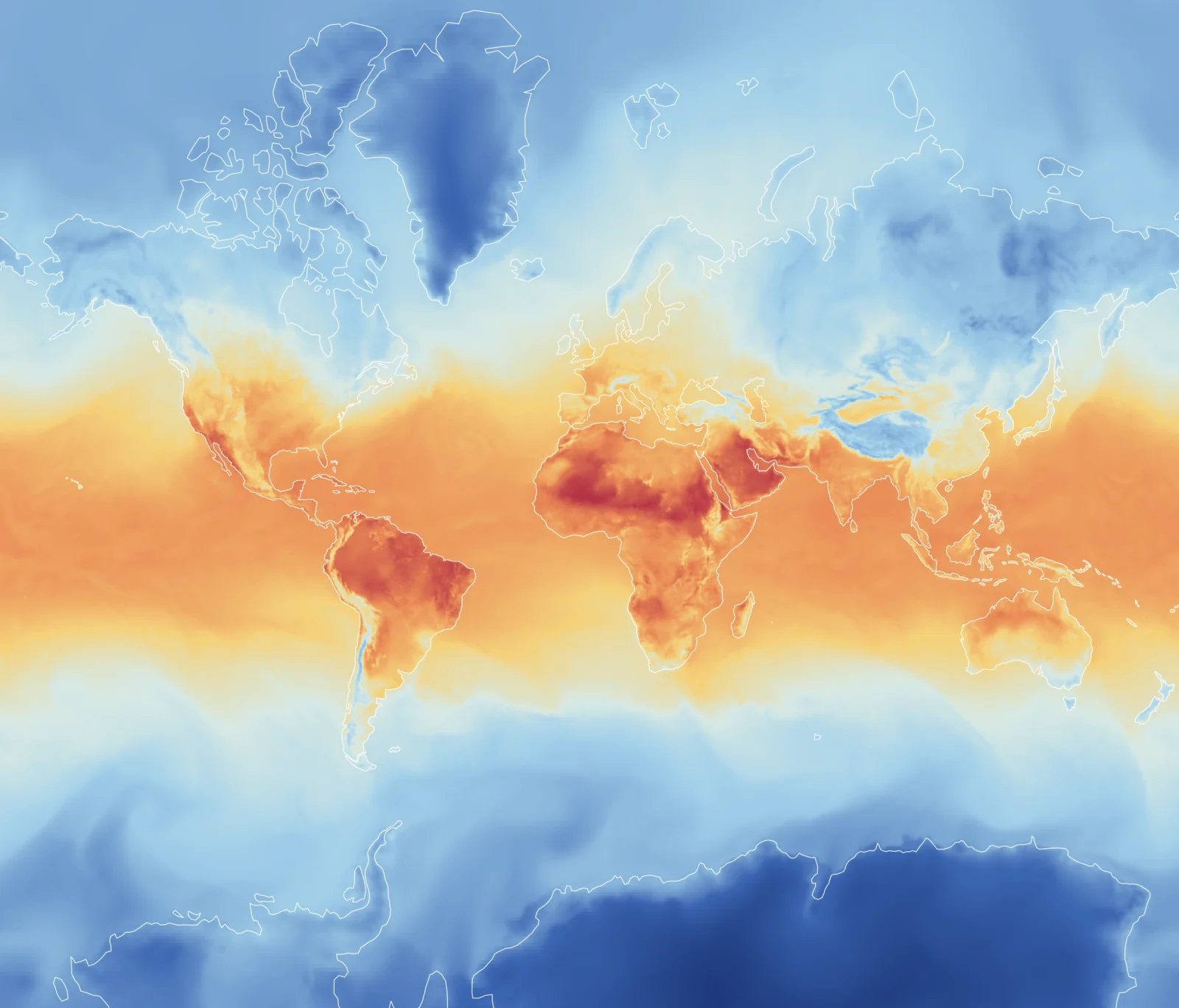
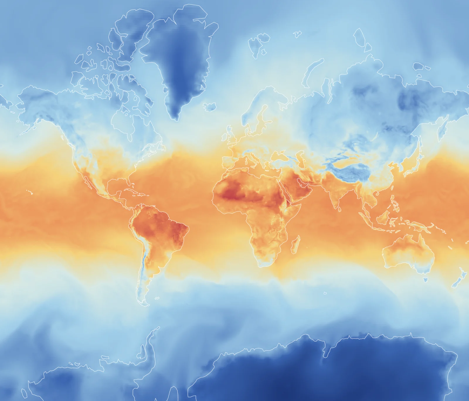
- Apply your calculation Subtract the minimum from the maximum at every grid cell.[max_temperature_2m_3h][max_temperature_2m_3h]- [min_temperature_2m_3h]- [min_temperature_2m_3h]
- Get a new weather field One output grid showing the three-hour temperature range.
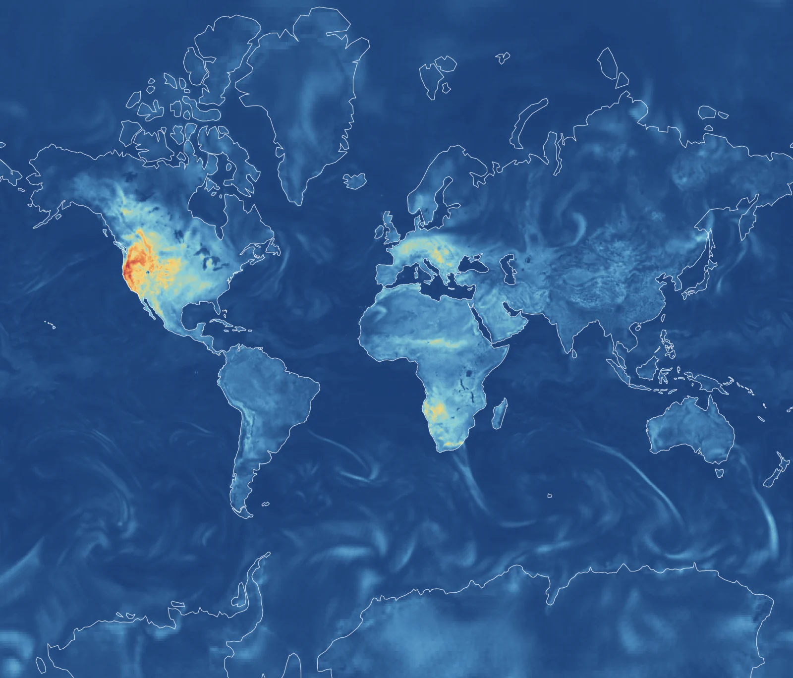
For example, subtracting the three-hour minimum temperature from the three-hour maximum gives the temperature range at each location. More detailed calculations can compare variables, average conditions over time, or combine pressure levels.
Available endpoints
Validate a calculation, calculate a grid, or generate threshold polygons.
| Validate Calculation | Check calculation syntax. Returns whether it is valid and any compiler errors, without checking forecast data availability. |
| Gridded Calculation | Calculate a weather field for selected forecast hours. Returns native-grid values as a Zarr v3 ZIP archive. |
| Threshold Calculation | Return GeoJSON polygons for selected forecast hours using a fixed-value or percentile threshold. |
The calculation and polygon endpoints currently support WeatherMesh 6 global and 3 km CONUS. They check that the required forecast data is available when you run the calculation.
1. Setup
For a gridded calculation, send the following request parameters:
| Parameter | Description |
|---|---|
| model Required | The forecast model: wm-6 for global forecasts or wm-6-3km for 3 km CONUS forecasts. |
| initialization_time Required | The forecast initialization time. Use an ISO 8601 timestamp. |
| calculation Required | Calculation text describing the operation to run at each grid cell. |
| forecast_hours Optional | A single integer selects one forecast hour; a list selects specific hours. Omit to evaluate all available forecast hours. |
| lat_range Optional | Southern and northern bounds, written as [south, north] . Omit to use the full latitude range. |
| lon_range Optional | Western and eastern bounds, written as [west, east] . A west value greater than east selects across the dateline. Omit to use the full longitude range. |
For requests with multiple forecast hours, each hour is calculated separately. Hours that don’t have all the required input data are omitted from the result and reported in anchor_errors . Results for the remaining hours are still returned. If every requested hour fails, the request returns an error.
In the example below, the calculation finds the maximum temperature over the next 72 hours at each grid cell. The input covers hours 0–360, so output grids can be calculated for hours 0–288. Later hours are skipped because their 72-hour window extends beyond the available input.
Hour 12 · Inputs 12–84h (25 samples) → 1 gridNo grid generated, less than 72 hours available.
The output uses the same grid as the input data. When you set lat_range and lon_range on a supported grid, only data for that area is loaded and calculated. The output may include extra cells around the edges.
2. Variables
Forecast variables are lowercase snake_case references enclosed in square brackets. A reference without selectors, such as [temperature_2m] , uses the ensemble mean. Selectors inside the brackets choose a distribution, level, or member; for example, [temperature_2m(members=42)] selects ensemble member 42. Forecast inputs retain their native units.
See Variables for the variables and pressure levels available for a model. Its distribution_details field shows whether each variable supports deterministic, percentile, threshold-probability, or ensemble-member selections. Custom Calculations use the forecast variable values in their documented native units and do not convert them automatically.
| Reference | Syntax |
|---|---|
| Mean | [temperature_2m] |
| Standard deviation | [temperature_2m(std)] |
| Deterministic | [temperature_2m(det)] |
| Single ensemble member | [temperature_2m(members=42)] |
| All ensemble members | [temperature_2m(members)] |
| Upper-air levels | [temperature(level=850)] [temperature(level=[850, 700, 500])] [temperature(levels=[850, 700, 500])] |
| Percentile | [temperature_2m(p90)] |
| Threshold probability | [total_precipitation_3h(gt_0p25mm)] |
| Precipitation-type probability | [p_type(p_snow)] |
2.1 Accumulated variable timing
Variables like [snowfall_3h] and [total_precipitation_3h] represent totals over the three hours ending at their valid time rather than values at a single instant. A value valid at 06:00 therefore covers 03:00–06:00. The calculation language uses the API's valid time directly and does not shift these variables.
3. Arithmetic operators and precedence
Calculations support these basic math operations:
- Add values with +
- Subtract values with -
- Multiply values with *
- Divide values with /
- Keep a value’s sign with +value , or reverse it with -value
- Group calculations with parentheses: (expression)
Calculations follow Python’s usual order: parentheses and function calls first, then positive or negative signs, multiplication and division, and finally addition and subtraction. Operations with the same priority run from left to right.
Here, multiplication happens before addition:
Use parentheses to change the order. Here, addition happens first:
You can combine arithmetic with functions:
To calculate a reciprocal, divide 1 by the value:
Floor division ( // ), modulo ( % ), bitwise operators, and shortcuts such as += are not supported. Use = for assignments, explained in section 4. Calculations do not support loops, imports, or other Python statements.
4. Calculation structure and evaluation
The last expression in a calculation describes the expected result at each grid cell, forecast hour, and selected pressure level.
A calculation must include at least one forecast variable, which defines the grid to calculate on. Expressions containing only numbers, such as 2 or tan(radians(45)) , pass syntax validation but cannot be calculated.
Numbers in a calculation apply to every input value. For example, the following expression subtracts 2 from the temperature at every grid cell and forecast hour:
When an expression contains multiple forecast variables, they are matched by location and valid time before the calculation is performed:
A calculation may contain zero or more assignments followed by a final expression. Each assignment binds a lowercase snake_case name to an expression so it can be reused later in the calculation. Assigned names are bare identifiers; square brackets identify forecast references.
Every assignment ends with a semicolon. Line breaks are formatting whitespace and do not separate statements.
Assignments are evaluated from left to right. You can assign a name more than once. A reassignment uses the name’s previous value to calculate its new value. Later references use the new value, while earlier assignments keep the expression they originally captured. You cannot use a name before it has been assigned, including in its own first assignment.
This constant-only example illustrates assignment syntax; execution still requires a forecast reference:
4.1 Multi-level expressions
An upper-air variable without a level= selector returns one grid for each available pressure level. Select one level, such as level=850 , to get a single grid. Use a list like level=[850, 700, 500] to get a separate grid for each of those levels.
The examples below show how different level selections affect the result:
| Formula | Result |
|---|---|
| [temperature] | One grid for each available pressure level. |
| [temperature(level=850)] | One temperature grid at 850 hPa. |
| [temperature] - [temperature_2m] | Subtracts surface temperature from temperature at each pressure level. Returns one grid per level. |
| [temperature] - [dewpoint(level=700)] | Subtracts the same 700 hPa dewpoint grid from temperature at each pressure level. Returns one grid per level. |
| [temperature(level=850)] - [dewpoint(level=850)] | One grid showing temperature minus dewpoint at 850 hPa, calculated at each grid cell. |
| [temperature(level=[850, 700, 500])] - [dewpoint(level=[850, 700, 500])] | Three grids showing temperature minus dewpoint at 850, 700, and 500 hPa. Both lists must contain the same levels in the same order. |
| [temperature(level=[850, 700, 500])] - [dewpoint(level=[500, 700, 850])] | Fails with LEVEL_ALIGNMENT_MISMATCH because the levels are in a different order. Levels are not reordered automatically. |
| [temperature(level=850)] - [dewpoint(level=700)] | One grid showing temperature at 850 hPa minus dewpoint at 700 hPa. Single-level inputs can use different pressure levels. |
5. Core functions
Core functions take numbers, forecast variables, or calculations as inputs. They calculate a result separately at each grid cell.
To combine values across pressure levels, time, or ensemble members, use aggregate_level(...) , aggregate_time(...) , or aggregate_members(...) , explained in section 9. Each uses min , max , sum , or mean to choose how the values are combined.
Core functions do not combine values from different locations.
5.1 Comparing and combining values
| Function | Description | Example and result |
|---|---|---|
| min(a, b, ...) | Returns the smallest input. | min([temperature_2m], [temperature_2m(det)])min([temperature_2m], [temperature_2m(det)]) Selects the lower of the mean and deterministic temperature at each point and time. min([temperature_2m] - 273.15, 30) can also cap a Celsius result at 30. |
| max(a, b, ...) | Returns the largest input. | max([temperature_2m] - 273.15, 0)max([temperature_2m] - 273.15, 0) Converts negative temperatures to 0 while leaving positive temperatures unchanged. |
| sum(a, b, ...) | Adds two or more inputs at each point and time. | sum([wind_u_10m], [wind_v_10m], 2)sum([wind_u_10m], [wind_v_10m], 2) Adds the two wind-component values and 2 at each grid cell. Inputs of 3, 4, and 2 produce 9. |
| mean(a, b, ...) | Averages the input values. | mean([temperature_2m], [temperature_2m(det)])mean([temperature_2m], [temperature_2m(det)]) Averages the mean and deterministic temperature at each point and time. |
5.2 Scores and limits
| Function | Description | Example and result |
|---|---|---|
| clamp(value, lower, upper) | Limits a value to a specified range. | clamp([temperature_2m] - 273.15, 0, 30)clamp([temperature_2m] - 273.15, 0, 30) Restricts the result to 0–30: −5 becomes 0, 18 remains 18, and 35 becomes 30. |
| clamp01(value) | Limits a value to the range from 0 to 1. | clamp01([total_precipitation_3h] / 10)clamp01([total_precipitation_3h] / 10) 0 mm becomes 0, 5 mm becomes 0.5, and 10 mm or more becomes 1. Equivalent to clamp(value, 0, 1) . |
| band(value, lower, upper) | Converts a value into a linear score from 0 to 1. | band([temperature_2m], 283.15, 298.15)band([temperature_2m], 283.15, 298.15) 283.15 K becomes 0, 290.65 K becomes 0.5, and 298.15 K or more becomes 1. Equivalent to clamp01((value - lower) / (upper - lower)) . |
| step(edge, value) | Converts a threshold into 0 or 1. | step(273.15, [temperature_2m])step(273.15, [temperature_2m]) Temperatures below 273.15 K become 0 and temperatures at or above 273.15 K become 1. |
| mix(a, b, weight) | Mixes two values using a weight. | mix([temperature_2m], [temperature_2m(det)], 0.25)mix([temperature_2m], [temperature_2m(det)], 0.25) Uses 75% of the mean and 25% of the deterministic temperature. Equivalent to a * (1 - weight) + b * weight ; 0 returns a and 1 returns b . |
5.3 Math functions
| Function | Description | Example and result |
|---|---|---|
| abs(value) | Returns the absolute value. | abs([temperature_2m] - [temperature_2m(det)])abs([temperature_2m] - [temperature_2m(det)]) Measures the difference between two forecasts, regardless of which is higher. Inputs of 20 and 17 produce 3 in either order. |
| sqrt(value) | Returns the square root. | sqrt(max([cape], 0))sqrt(max([cape], 0)) The max protects against negative inputs, and a CAPE value of 900 produces 30. |
| hypot(a, b) | Returns the hypotenuse of two values. | hypot([wind_u_10m], [wind_v_10m])hypot([wind_u_10m], [wind_v_10m]) Combines perpendicular components; inputs 3 and 4 produce 5. |
| pow(value, exponent) | Raises a value to a power. | pow([wind_speed_10m], 2)pow([wind_speed_10m], 2) An input of 4 and exponent of 2 produce 16. |
| exp(value) | Returns e raised to the input value. | exp([wind_speed_10m] / 10)exp([wind_speed_10m] / 10) Applies the exponential function at each point and time. An argument of 0 produces 1; an argument of 1 produces approximately 2.71828. |
| ln(value) | Returns the natural logarithm of a positive value. | ln(max([wind_speed_10m], 0.001))ln(max([wind_speed_10m], 0.001)) The max keeps the argument positive. ln(1) produces 0, and ln(2.71828) produces approximately 1. |
5.4 Angles and trigonometry
| Function | Description | Example and result |
|---|---|---|
| sin(value) | Returns the sine of an angle in radians. | sin(radians(30))sin(radians(30)) 30 degrees produces 0.5. |
| cos(value) | Returns the cosine of an angle in radians. | cos(radians(60))cos(radians(60)) 60 degrees produces 0.5. |
| tan(value) | Returns the tangent of an angle in radians. | tan(radians(45))tan(radians(45)) 45 degrees produces 1. |
| asin(value) | Returns the inverse sine as an angle in radians. | asin(clamp([wind_v_10m] / 10, -1, 1))asin(clamp([wind_v_10m] / 10, -1, 1)) The example keeps the argument between −1 and 1. An argument of 0.5 produces approximately 0.5236 radians, or 30 degrees. |
| acos(value) | Returns the inverse cosine as an angle in radians. | acos(clamp([wind_u_10m] / 10, -1, 1))acos(clamp([wind_u_10m] / 10, -1, 1)) The example keeps the argument between −1 and 1. An argument of 0.5 produces approximately 1.0472 radians, or 60 degrees. |
| atan(value) | Returns the inverse tangent as an angle in radians. | atan([wind_u_10m] / 10)atan([wind_u_10m] / 10) An argument of 1 produces approximately 0.7854 radians, or 45 degrees. |
| atan2(a, b) | Returns an angle in radians using the two-argument inverse tangent. | atan2([wind_v_10m], [wind_u_10m])atan2([wind_v_10m], [wind_u_10m]) Calculates an angle from both wind-component inputs, taking their signs into account. Inputs of 1 and 1 produce approximately 0.7854 radians, or 45 degrees. |
| radians(value) | Converts degrees to radians. | radians(180)radians(180) 180 degrees produces approximately 3.14159 radians. |
| degrees(value) | Converts radians to degrees. | degrees(3.141592653589793)degrees(3.141592653589793) π radians produces 180 degrees. |
5.5 Rounding
| Function | Description | Example and result |
|---|---|---|
| floor(value) | Rounds a value down. | floor([temperature_2m])floor([temperature_2m]) An input of 18.9 produces 18. |
| ceil(value) | Rounds a value up. | ceil([temperature_2m])ceil([temperature_2m]) An input of 18.1 produces 19. |
| round(value) | Rounds a value to the nearest integer. | round([temperature_2m])round([temperature_2m]) An input of 18.6 produces 19. Values ending in .5 round away from zero: 2.5 becomes 3, and −2.5 becomes −3. |
You can use functions inside other functions and combine them with math operators. This example combines warm temperatures and calm winds into a mosquito-suitability score:
Use the function names and inputs listed above. Version 1 does not support custom functions.
6. Conditional expressions
Use if / else to choose between two results. If the condition is true, the calculation uses the first result. Otherwise, it uses the result after else . Every if needs an else .
This example converts temperature to Celsius, then replaces temperatures below zero with 0 :
You can compare values using < , <= , > , >= , == , and != . You cannot combine conditions with and or or .
6.1 Checking for finite values
Use is_finite(value) to check whether a value is a regular number. It returns false for missing or undefined values ( NaN ) and positive or negative infinity. It checks each grid cell without changing its value.
This example keeps regular temperature values and replaces all others with 0 :
7. Selecting another forecast
The request parameter forecast_hours chooses which output hours to calculate. The selectors in this section choose which forecast data a variable reads while each output hour is calculated.
By default, a variable uses data for the forecast hour being calculated. Time selectors let you choose another hour or a list of hours from the same forecast run. Selecting one hour gives one grid that you can use directly in a calculation. Selecting several hours keeps their grids separate; you can combine them, pick one, or calculate with another input that uses the same hours in the same order.
Use offset_hours to select hours relative to the hour being calculated. For example, offset_hours=24 selects 24 hours later, and offset_hours=-6 selects 6 hours earlier. A list such as offset_hours=[-6, 0, 6] selects all three times.
Use forecast_hour to select hours counted from forecast_zero . The valid time is forecast_zero + forecast_hour ; forecast_zero can differ from initialization_time . See Run Information for a run's forecast_zero and available hours. For example, forecast_hour=24 always selects hour 24. It also accepts a list of hours. You cannot use offset_hours and forecast_hour together in the same variable reference.
| Selector | Time selected |
|---|---|
| [temperature_2m(offset_hours=24)] | 24 hours after the hour being calculated |
| [temperature_2m(offset_hours=-6)] | 6 hours before the hour being calculated |
| [temperature_2m(offset_hours=[-6, 0, 6])] | 6 hours before, the current hour, and 6 hours after, in that order |
| [temperature_2m(forecast_hour=0)] | Hour 0 of the forecast run |
| [temperature_2m(forecast_hour=[0, 12, 24])] | Hours 0, 12, and 24 of the forecast run, in that order |
Selecting one hour gives one grid, so you can use it directly in a calculation. This example calculates the temperature change over the next 24 hours:
You can also combine time and distribution selectors in a function. This example picks the higher of the 90th-percentile temperature 24 hours later and the mean temperature at the current hour:
Selecting a list keeps each hour’s grid separate:
For a calculation at hour 12, this selects temperature at hours 6, 12, and 18, returning three grids in that order. The next section explains how to work with these layers.
8. Working with multi-grid results
A calculation can return multiple grids. For example, it may return one grid for each selected pressure level or forecast hour. The following functions let you arrange grids in a specific order, select a grid by its pressure level or time, or aggregate multiple grids into one result. Each function processes every grid cell separately.
| Function | Description |
|---|---|
| stack(first, ...) | Combines results into an ordered stack of layers |
| pressure_layer(value, index) | Selects one pressure layer by its index, starting at 0 |
| time_layer(value, index) | Selects one time layer by its index, starting at 0 |
| reduce(value, operation) | Combines all layers into one grid, calculating a value at each grid cell |
8.1 Stack results
Use stack(first, ...) to combine results into an ordered stack of separate grids.
This creates two grids: temperature at 850 hPa, followed by dewpoint at 700 hPa. Each grid keeps its own values.
8.2 Select a pressure layer
Use pressure_layer(value, index) to select one pressure layer from a result. Indices start at 0 and follow the order of the selected levels.
This calculates temperature minus dewpoint at two pressure levels and three times. Index 1 selects the result at 500 hPa, keeping all three times.
8.3 Select a time layer
Use time_layer(value, index) to select one time layer from a result. Indices start at 0 and follow the order of the selected times.
This calculates the temperature change from the current hour at two pressure levels for offsets 0, 6, and 12 hours. Index 1 selects the change after 6 hours, keeping both pressure levels.
8.4 Reduce layers
Use reduce(value, operation) to combine values across all times and vertical levels into one grid. The calculation happens separately at each grid cell.
This example finds the highest temperature at each grid cell across two vertical levels and two times: 850 and 500 hPa, at the hour being calculated and 6 hours later.
Choose min , max , sum , or mean as the operation. For example, reduce(value, mean) averages values across all times and vertical levels at each grid cell. Write the operation name without parentheses; mean(a, b) is a separate function that averages its inputs.
To combine only vertical levels while keeping times separate, use aggregate_level(...) in section 9.1. To combine values across time, use aggregate_time(...) in section 9.2. To combine ensemble members while keeping times separate, use aggregate_members(...) in section 9.3.
9. Aggregate across levels, times, or members
Aggregation takes multiple values at each grid cell and produces one result. It can work across any one of three dimensions: pressure levels, times, or ensemble members.
Each aggregation uses a value and an operation . Choose min , max , sum , or mean to control how the values are combined.
| Function | What it combines |
|---|---|
| aggregate_level(...) | Pressure levels |
| aggregate_time(...) | Selected times or a time window |
| aggregate_members(...) | All ensemble members |
9.1 Pressure levels
Use aggregate_level(value, operation) to combine values across pressure levels at each grid cell. It returns one grid for each selected time.
You can combine all levels in the input or specify a pressure range using aggregate_level(value, operation, level_start, level_end) .
| Argument | Meaning |
|---|---|
| level_start | One end of the pressure range, in hPa |
| level_end | The other end of the pressure range, in hPa |
Both ends of the range are included. Write the pressure bounds as numbers, rather than variables or calculations.
The range must stay within the available pressure levels and include at least one level. Invalid ranges reject the request. If a level inside the range is missing, it is left out. The range is not shortened automatically.
| Syntax | Result |
|---|---|
| aggregate_level([temperature], max) | Highest temperature across all available pressure levels |
| aggregate_level([temperature(level=[850, 700, 500])], max) | Highest temperature across 850, 700, and 500 hPa |
| aggregate_level([temperature], max, 500, 850) | Highest temperature across available levels from 500 to 850 hPa, including both ends |
9.2 Time
Use aggregate_time(value, operation, hours_before, hours_after) to combine values across a time window at each grid cell. Both ends of the window are included.
If the input already selects a list of times, use aggregate_time(value, operation) to combine those times.
| Argument | Meaning |
|---|---|
| hours_before | How many hours before the hour being calculated the window starts |
| hours_after | How many hours after the hour being calculated the window ends |
Use 0 to start or end the window at the hour being calculated. Write both bounds as whole numbers of zero or more. Fractions, variables, calculations, and decimal forms such as 6.0 are not supported.
The calculation includes every available input sample within the window. A variable’s own time coverage stays the same: each value of [total_precipitation_3h] still represents a three-hour total.
| Syntax | Result |
|---|---|
| aggregate_time([temperature_2m], max, 0, 72) | Highest temperature from the hour being calculated through 72 hours later |
| aggregate_time([temperature_2m], max, 12, 36) | Highest temperature from 12 hours before through 36 hours after the hour being calculated |
| aggregate_time([temperature_2m], max, 24, 0) | Highest temperature over the previous 24 hours, including the hour being calculated |
| aggregate_time([temperature_2m(offset_hours=[-6, 0, 6])], max) | Highest temperature across the three selected times: 6 hours before, the current hour, and 6 hours later |
9.3 Members
Use aggregate_members(value, operation) to combine values across all ensemble members at each grid cell. It returns one grid for each selected time.
The input must use the members selector so the calculation contains all available ensemble members.
Member aggregation uses every ensemble member available for the selected model and initialization time. To use one member without aggregating, select it directly, such as [temperature_2m(members=42)] .
| Syntax | Result |
|---|---|
| aggregate_members([temperature_2m(members)], mean) | Average temperature across all ensemble members |
10. Errors
Invalid calculations or level selections reject the request. For requests with multiple forecast hours, hours without all the required input data are skipped. Results are returned for the remaining hours.
Errors identify the affected expression and show the available pressure levels or forecast hours when relevant.
| Error | Condition |
|---|---|
| INVALID_CALCULATION | The calculation contains invalid syntax or uses an unsupported operation. The request is rejected |
| INVALID_LEVEL_SELECTION | A pressure-level selection is empty or incorrectly written. The request is rejected |
| LEVEL_UNAVAILABLE | A selected pressure level is unavailable for the variable. Missing levels are not estimated. The request is rejected |
| LEVEL_ALIGNMENT_MISMATCH | Inputs use different pressure levels or list them in a different order. Levels are not matched or reordered automatically. The request is rejected |
| INVALID_TIME_WINDOW | hours_before or hours_after is not a whole number of zero or more. Write numbers directly; fractions, variables, calculations, and decimal forms such as 6.0 are not supported. The request is rejected |
| FORECAST_HOUR_UNAVAILABLE | A selected hour is unavailable in the forecast run. Values between available hours are not estimated. The affected calculation hour is skipped |
| FORECAST_SELECTION_FAILED | None of the requested forecast hours could be calculated. The individual failures are returned in anchor_errors |
| INCOMPLETE_TIME_WINDOW | The window extends beyond the available forecast data. It is not shortened automatically. The affected calculation hour is skipped |
| MISSING_INPUT_DATA | A required variable is missing at an input hour. The affected calculation hour is skipped |